Does Google Sheets have a built-in Gantt chart?

There is no Gantt chart type in the chart editor. The usual workarounds are a stacked bar chart with an invisible first series, or conditional formatting that colours cells on a row of dates.

Which method is better, the bar chart or conditional formatting?

The bar chart is quicker for a picture to paste into a report. Conditional formatting stays inside the grid, so it is easier to read next to the task list, to print and to extend with a today line, weekends or % done.

Why do my bars start in the year 1899?

The chart is treating your start dates as numbers counted from Google Sheets' base date. Chart a start offset (start date minus project start) instead of the raw date, or set a minimum on the horizontal axis.

Can a Google Sheets Gantt chart handle dependencies?

Not by itself. Both methods draw whatever dates you type. To move later tasks when an earlier one slips, you need formulas that calculate each start date from its predecessor's finish date.

How to make a Gantt chart in Google Sheets (2 methods)

Google Sheets has no Gantt chart type, so you build one. Either make a stacked bar chart from a start-offset column and a duration column and hide the first series, or lay out a row of dates and colour each task's cells with a conditional formatting custom formula such as =AND(D$1>=$B2, D$1<=$C2).

A Gantt chart is a bar chart of a schedule: one row per task, time running left to right, and a bar from each task's start to its finish. Google Sheets does not offer it as a chart type, but two standard tricks get you there. Method A uses the chart editor. Method B uses conditional formatting in the cells themselves.

Both methods start from the same task list.

Set up the task list

Put one task per row, starting in row 2:

	A	B	C
1	Task	Start	End
2	Kick-off	(date)	(date)
3	Requirements	(date)	(date)
4	Design	(date)	(date)

Type real dates in columns B and C (Format > Number > Date if Sheets shows numbers). Keep the tasks in the order you want them to appear on the chart.

Method A: a stacked bar chart

The idea: each bar is two stacked pieces. The first piece runs from the project start to the task start and is made invisible. The second piece is the task's duration, and that is the bar you see.

Add two helper columns. In D1 type Start offset and in E1 type Duration. In D2 enter =B2-$B$2 (days from the project start, assuming the first task starts the project). In E2 enter =C2-B2+1 (the task's length in days, counting both the start and end day). Fill both formulas down.
Select the data for the chart. Select A1:A4, then hold Ctrl (Cmd on a Mac) and select D1:E4, so the chart gets the task names, the offset and the duration.
Insert the chart. Go to Insert > Chart. In the chart editor, on the Setup tab, set Chart type to Stacked bar chart. Google's bar chart help describes stacked bar charts as needing at least two data series, which is exactly what the offset and duration columns are.
Hide the offset series. Open the Customize tab > Series, pick the Start offset series and set its fill opacity to 0% (or its colour to none). The bars now float, starting on each task's start day.
Tidy the chart. Under Customize > Chart & axis titles, add a title. Turn off the legend under Legend if you don't need it. Under Series you can also add data labels to show each duration.
Check the order. Tasks should read from top to bottom in the order of your list. If your version shows them reversed, sort the source rows the other way.

Why the offset column? If you chart the raw dates, Sheets treats them as numbers counted from its base date, and every bar starts decades before your project. Charting days from the start avoids that. The cost is that the horizontal axis shows day numbers, not calendar dates.

Method B: conditional formatting on a date grid

The idea: turn the cells to the right of the task list into a calendar, and colour each cell whose date falls between the task's start and end.

Build the date row. In D1 enter =$B$2 (the first task's start). In E1 enter =D1+1. Fill E1 to the right for as many days as the project needs. Format row 1 as a short date (Format > Number > Custom date and time, for example day and month), then narrow the columns so each day is a thin cell.
Select the grid. Select from D2 across to the last date column and down to the last task row.
Open the rules panel. Go to Format > Conditional formatting. Under "Format cells if", choose Custom formula is.
Enter the bar formula:

=AND(D$1>=$B2, D$1<=$C2)

The dollar signs matter. D$1 locks the row, so every cell compares against the date in row 1 of its own column. $B2 and $C2 lock the columns, so every cell compares against the start and end in its own row. Google's help page on conditional formatting explains this use of absolute references.
Pick a fill colour and click Done. Each task now shows a coloured bar across its dates.
Add more rules (optional). Click "Add another rule" with the same range:
- Weekend shading: =WEEKDAY(D$1,2)>5 with a light grey fill.
- Today line: =D$1=TODAY() with a red fill.
- Milestones: if you add a Type column, a rule that checks it can colour milestone days differently.

Rule order matters. Google's help states that rules are evaluated in the order listed and the first rule that is true sets the format. Put the today line above the bar rule if you want it to cut through the bars, and put weekend shading below the bar rule if bars should stay solid on weekends.

Adding % done. Add a column for % done (for example column F with values from 0 to 1, and start the date grid one column further right). A darker rule placed above the bar rule, such as =AND(G$1>=$B2, G$1<$B2+($C2-$B2+1)*$F2) with the grid starting in column G, shades the completed part of each bar.

The limits of both methods

These charts draw the dates you type. They don't plan anything.

No dependencies. If the design task slips three days, every task that waits for it stays where it was until you retype its dates. Real scheduling needs each start date to be calculated from its predecessor's finish, and that needs more formulas than a chart can hold.
Calendar days, not working days. =C2-B2+1 counts weekends and public holidays. You can switch to NETWORKDAYS and WORKDAY, but then you have to maintain a holiday list and make sure every formula uses it.
No workload view. A Gantt bar says nothing about who does the work. You won't see that one person has three overlapping tasks in the same week unless you build a separate resource table.
No status. Neither method tells you whether a task is behind plan on a given date. You read that by eye.
Upkeep. Method A breaks when rows are inserted outside the chart range. Method B needs the grid extended by hand when the project runs longer.

For a short task list these limits are fine. For a project you will update every week, the manual work adds up.

An Excel alternative

Both methods above are for Google Sheets and need no template. If you use Excel, our Gantt Chart Project Planner handles those limits with formulas. It is an Excel workbook (.xlsx) with no macros. Scripts recalculated it in Excel for Mac 16.114.3 and LibreOffice. It has not been tried in Google Sheets, so we do not sell it for use there.

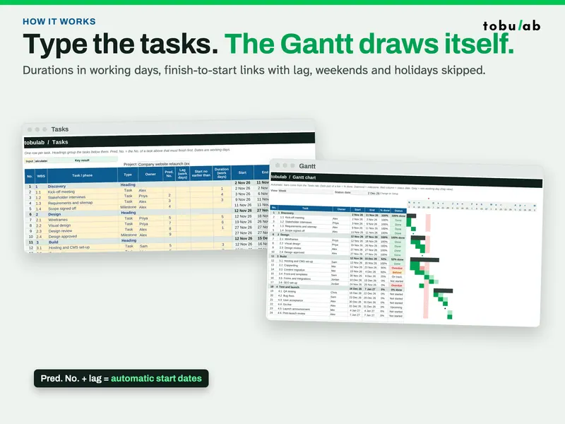
Calculated dates. Type each task with a duration in working days. Start and end dates are calculated, following your dependencies, weekends and holidays.
Real dependencies. Finish-to-start links to the task that must finish first, with lag or overlap.
Your working week. Mon-Fri, Mon-Sat, Sun-Thu, Sat-Wed or 7 days, plus your own holiday list, for any country.
Automatic Gantt chart. Day or week view, % done shading, milestones, today line and shaded non-working days. The bars are conditional formatting, the same idea as Method B, driven by the calculated dates.
Status updates itself. Done, On track, Behind, Overdue or Not started, compared with the plan on your status date. Phases roll up dates and % done from their tasks.
RAID log and resource load. Risks, assumptions, issues and dependencies with probability × impact scoring and overdue flags, and work days per person per week, red when someone is overloaded.
One-page dashboard. Actual vs planned progress, overdue tasks, upcoming milestones, phase progress and open risks.

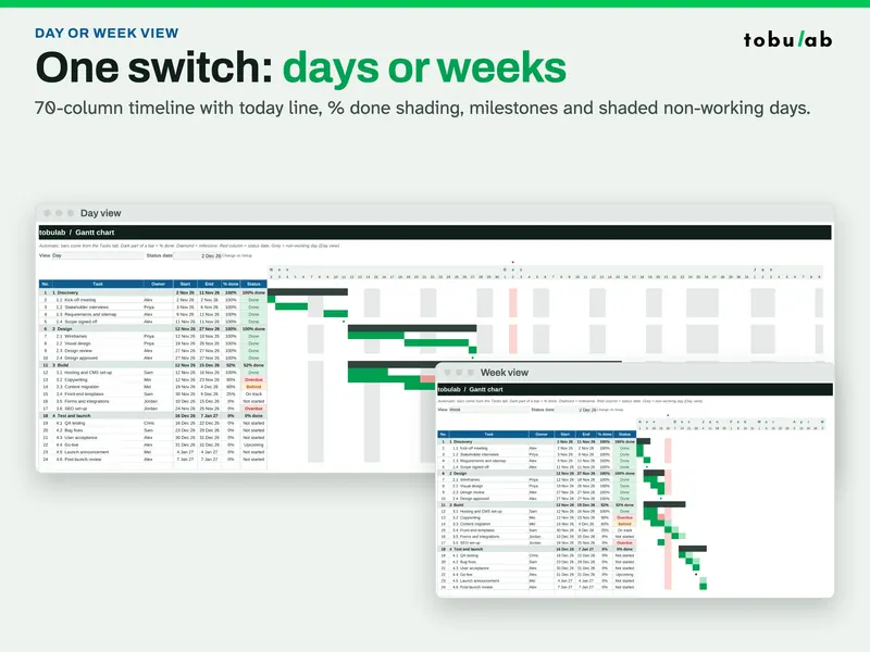
Gantt tab of the Excel planner with bars, % done shading, milestones and a status-date column, switchable between day and week view

The download has a filled example (a 4-phase website relaunch with 20 tasks and milestones and 6 people), a blank copy and a 4-page PDF quick-start guide. The Tasks tab has 150 rows and the Gantt covers 70 days or weeks.

Tasks tab where you type tasks, durations and predecessor numbers, next to the Gantt chart that draws itself

Questions

Does Google Sheets have a built-in Gantt chart?: There is no Gantt chart type in the chart editor. The usual workarounds are a stacked bar chart with an invisible first series, or conditional formatting that colours cells on a row of dates.
Which method is better, the bar chart or conditional formatting?: The bar chart is quicker for a picture to paste into a report. Conditional formatting stays inside the grid, so it is easier to read next to the task list, to print and to extend with a today line, weekends or % done.
Why do my bars start in the year 1899?: The chart is treating your start dates as numbers counted from Google Sheets' base date. Chart a start offset (start date minus project start) instead of the raw date, or set a minimum on the horizontal axis.
Can a Google Sheets Gantt chart handle dependencies?: Not by itself. Both methods draw whatever dates you type. To move later tasks when an earlier one slips, you need formulas that calculate each start date from its predecessor's finish date.

Sources

Updated 2026-10-26 · by tobulab